Optimisation of Partitioned Temporal Joins

Thomas Zurek

Department of Computer Science

University of Edinburgh

This is an HTML version of a talk that I gave on 8 July 1997 on the BNCOD'97 conference. I have merged the contents of the slides with the notes that I had prepared. For more details you will have to check the corresponding conference paper whose reference is here. This talk also gives a brief overview of my PhD project.

Table of Contents

• Slide 1: Overview
• Slide 2: Temporal Relations
• Slide 3: Temporal Joins
• Slide 4: Nested-Loops Temporal Join
• Slide 5: Symmetric Partitioning
• Slide 6: Difference with Conventional Joins
• Slide 7: A Partitioned Nested-Loops Temporal Join
• Slide 8: ...and using a different partition
• Slide 9: Summary of the Problems
• Slide 10: Optimisation Process
• Slide 11: Stage 1
• Slide 12: Stage 2
• Slide 13: Stage 3
• Slide 14: Elapsed Times for Optimisation
• Slide 15: Summary

Slide 1: Overview

1. temporal relations, temporal joins, temporal join conditions (slides 2, 3)
2. temporal join processing
   • nested-loops approach (slide 4)
   • symmetric partitioning (slides 5, 6, 7, 8, 9)
3. structure of the optimisation process (slides 10, 11, 12, 13, 14)
4. summary (slide 15)

Back to Table of Contents

Slide 2: Temporal Relations

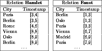
Hamlet and Faust are temporal relations that contain information on where and when plays are performed. They are said to be temporal relations because each tuple has a timestamp. Frequently, these timestamps are represented as intervals because intervals have proved to be the most versatile representation of time. They allow to express almost any time reference that we use in natural language.

Back to Table of Contents

Slide 3: Temporal Joins

This is an example for a temporal join. It would answer the query ``During what periods are both plays performed simultaneously?''. It is temporal because the join condition involves the timestamp attributes. The predicate, i.e. temporal intersection, is the procedural expression of simultaneity.

Back to Table of Contents

Slide 4: Nested-Loops Temporal Join

Processing Hamlet Faust as a nested-loops join.

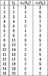
This is an illustration of the simplest algorithm for processing a join - and a temporal join in particular:

• one line per tuple of Faust
• one column per tuple of Hamlet
• lines and columns are labeled with the timestamp
• squares = tuple pairs that potentially qualify for the result
• all squares = search space

Back to Table of Contents

Slide 5: Symmetric Partitioning

Symmetric partitioning is a technique used for

• hash join processing, and
• parallel join processing.

It splits one, big operation into several, small and independent operations. For that purpose, each relation is partitioned into several fragments. Fragments are not created arbitrarily but on base of the join condition. This is the crucial point (see next slide).

with

Symmetric partitioning has two major advantages:

1. The subjoins are independent, i.e. they can be processed concurrently.
2. It can be considered as a kind of preprocessing that gets rid of some unnecessary work: e.g. those tuples in the first fragment of Hamlet are not compared with the tuples in the second and third fragments of Faust because those comparisons can be discarded.

Back to Table of Contents

Slide 6: Difference with Conventional Joins

Partitioned Equi-Joins

Partitioned Temporal-Joins

• Conventional equi-join conditions lead to disjoint fragments.
• Temporal join conditions usually require non-dsijoint fragments in which tuples are replicated.

Back to Table of Contents

Slide 7: A Partitioned Nested-Loops Temporal Join

This is an example of symmetric partitioning for a temporal join.

• Each fragment is associated with a certain interval of time domain.
• A tuple is put into a fragment if its timestamp intersects with that interval.
• Obviously there some tuples whose timestamp intersects with more than one partitioning interval. These tuples are assigned to more than one fragment, thus are replicated between fragments.
• This leads to several problems:
  • a possible effort on the replication itself,
  • the search space becomes bigger, i.e. there is more processing,
  • tuple replication leads to a replication of tuple comparisons; as a consequence, there can be duplicates in the result (red/dark squares).

Back to Table of Contents

Slide 8: ...and using a different partition

A (minimal) change of breakpoints delivers totally different scenario:

Back to Table of Contents

Slide 9: Summary of the Problems

Three types of overhead

• replication overhead: costs caused by the replication process itself
• processing overhead: costs caused by a larger search space
• duplicates overhead: costs for the removal/avoidance of duplicates

The choice of partition is critical!

Back to Table of Contents

Slide 10: Optimisation Process

This is the structure of the optimisation process: 4 stages (corresponding to the 4 grey boxes) for finding a ``good'' partition for processing a temporal join.

The remainder of the talk shows the results of each stage. Technical details on how to get these results can be found in the paper.

Back to Table of Contents

Slide 11: Stage 1

The result of the 1st stage is a kind of index structure, called an IP-table (IP = Interval Partitioning). In general, IP-tables describe the characteristics of a certain bag of intervals, e.g. of those that appear as timestamps in a temporal relation R. An example scenario is shown here: There is the time line; intervals are represented as bold bars.

The IP-table that corresponds to that is the following:

IP-Table for a Relation R

• 1st column: interval start- and endpoints
  
• 2nd column: number of intervals starting at the respective timepoint
  
• 3rd column: number of intervals overlapping the respective timepoint

E.g. at timepoint 8, there is 1 starting interval and 2 intervals overlapping (i.e. they include 8 but do not end at time 8).

In the optimiser that I have in mind, IP-tables for individual temporal relations are maintained as metadata in the catalog, i.e.\ they already exist at optimisation time. IP-tables can be merged & condensed (compressed).

Back to Table of Contents

Slide 12: Stage 2

This slide shows the result of the second stage of the optimisation process. Here, you see the result of 3 different strategies that partition the bag of intervals into 4 fragments respectively.

uniform strategy: uniform partition of the time line

underflow strategy: well balanced fragments

min.-overlaps strategy: minimises number of intervals that overlap the breakpoints

All these strategies can be efficiently implemented on the base of IP-tables.

Back to Table of Contents

Slide 13: Stage 3

Something like this is the result of the third stage of the optimisation process in which each partition is analysed for its cost implications.

The costs are calculated on the of

(a)

a cost model and

(b)

the IP-tables of the relations that participate in the join

The diagram shows the costs for a certain temporal join and the partitions produced by the partitioning strategies in the previous optimisation stage. In practice, there will be much more strategies involved. The cheapest partition is then used for processing the join.

Back to Table of Contents

Slide 14: Elapsed Times for Optimisation

This slide shows the elapsed times for the optimisation process for each of the 3 partitioning strategies. Optimisation was run on a 2-processor SS-20 computing server. The times prove that it is reasonable to spend a few seconds on the optimisation in order to reduce the join processing times.

Back to Table of Contents

Slide 15: Summary

• introduction to temporal relations and temporal joins,
• ...and processing them using explicit partitioning,
• description of an optimisation process that chooses a ``good'' partition,
• ...and how it can be efficiently implemented, namely by using IP-tables.
• IP-tables not only serve for that purpose but can also be used for
  • balancing temporal index trees or
  • temporal join selectivity estimation

Back to Table of Contents

About this document ...

Optimisation of Partitioned Temporal Joins

This document was generated using the LaTeX2HTML translator Version 96.1 (Feb 5, 1996) Copyright © 1993, 1994, 1995, 1996, Nikos Drakos, Computer Based Learning Unit, University of Leeds.

The command line arguments were:
latex2html -split 0 -t T. Zurek: Optimisation of Partitioned Temporal Joins -address Thomas Zurek, tz@dcs.ed.ac.uk talk.

The translation was initiated by Thomas Zurek on Fri Jul 11 16:04:02 BST 1997