This part of the HASE Dinero user guide is divided into four main sections, which can be jumped to by following the hyperlinks below:
| How to Use HASE Dinero | |
| How the CPU Address is Split Into Separate Components | |
| The Principle of Locality | |
| How the Cache Utilisation is Calculated | |
| How the Miss Breakdown is Calculated |
Whilst it should be possible to use HASE Dinero with Linux HASE, a description for NT HASE only is supplied below as, at the time of writing, Linux HASE was still under development.
The first thing to do is get access to a PC running Windows NT with HASE installed. Once NT HASE is up and running, the Dinero project can be loaded. The Dinero project is downloadable from this website here. Extract the contents of the zip-file to a directory on your computer called dinero. Now open the file called dinero.edl (inside the dinero directory), using a standard text editor and alter the project directory string at the top of the file to point to the location of the dinero directory.
NT HASE also requires that you create a directory called "results" inside the dinero directory.
Now load HASE and select the Load Project option from the File menu. Browse your computer from within the open window that pops-up and locate the dinero directory, then double-click on the dinero.edl file inside it. This should load Dinero into HASE.
Note that you can change the level of hierarchy at which the cache architecture is viewed by right-clicking on the Level 1 Cache component and toggling the hierarchical level using the expand and up-level commands, but this can only be done whilst HASE is in Design mode.
Before HASE Dinero is ready to be used, the required object files must first be built. To do this, click on the Build button at the top of the HASE screen. Next go to the Build menu at the top of the screen and click on Generate Trace. This operation could take quite some time, depending on the speed of your computer.
To begin using HASE Dinero, click on the Simulate button at the top of the screen, then proceed to the next section.
HASE Dinero has several tutorial modes that demonstrate both cache operation and the principles of cache design. To begin using the tutorials, click here.
Modifying Simulation Parameters
If you do not wish to use the HASE tutorials, ensure that the Simulation Mode option of the Simulation Control window is set to Normal. This can be done by right-clicking on the Simulation Control screen and selecting Simulation Parameters from the pop-up list. This will load a window displaying all of the parameters of the Simulation Control window and allow you to modify them as desired.
Note that the above principle applies to all of the HASE Dinero windows.
Animated Mode vs. Fast Mode
HASE Dinero has two modes of operation: Animated and Fast.
In Animated mode, all simulation activity is visualised during simulation playback, but there is a 500 line trace file processing limit. Animated mode is intended so that an understanding of cache operation can be gained by viewing how cache hits and misses are determined and the effect that varying the cache configuration has on this process.
Fast mode is far more efficient than Animated mode, allowing up to 10,000,000 trace file lines to be processed, but there is no animation of simulation activity, with only the results entity being updated. In order to gain accurate simulation results, at least 1 million trace file references must be processed. Hence Fast mode provides a way to experiment with the actual expected performance of a cache configuration.
An Example Simulation Run
The final stage in understanding how to use HASE Dinero is running a simulation. Before a simulation can be run, certain of the HASE Dinero parameters must be changed from their default values. To run this example simulation, first change the following parameters in the Basic Cache Control window:
| Unified Cache Size: 64 | |
| Block Size: 4 |
This specifies that the cache should be able to contain 64 bytes of information in 16 lines each containing 4 bytes.
Now select the Run Simulation option from the Simulate menu at the top of the screen. Once the simulation has completed, go back into the Simulate menu and click on Animate. On the pop-up screen that appears, click on the Change button and then double click on the tracefile.trace file inside the results sub-directory. This will load the simulation results into memory.
It will be useful to observe how the contents of the unified cache change during simulation. To open the unified cache contents window, right click on the cache memory entity and choose View->Unified Cache Contents from the pop-up menu.
You are now ready to run the simulation, to do this simply click the play button on the Animation window that was opened earlier. Note that both the status window and results window update as a result of simulation activity, a full description of the information shown in these windows, and of all modifiable parameters in HASE Dinero can be found in the Point and Click Guide.
Note that the principle for running a simulation in Fast mode is the same as for Animated mode, with the only unclear point being that the results trace file must be both loaded and played before the results window will be updated.
Hopefully you now have all the information you need to use HASE Dinero. To gain an understanding of both cache operation and techniques that can be used to improve cache performance, the book Computer Architecture: A Quantitative Approach by J. Hennessy & D. Patterson comes highly recommended.
It is essential to understand the principles behind associative sets of cache lines before the address division method can be understood.
A cache is divided into a number of cache lines, each of which can hold one or more CPU words. The data storage capacity of each cache line is called a Block, and is expressed in bytes in HASE Dinero.
Every time a block is loaded to the cache, there is a finite number of lines that the cache control unit can decide to load the cache line to. If the cache is fully associative then the loaded block can be stored in any line in the cache. If the cache is x-way set associative then the cache is divided into separate sets, each set of which has x cache lines allocated to it. The loaded block can be stored on any of the lines in just one of the associative sets. If the cache is direct mapped then there is only 1 line in the entire cache that the block can be stored in.
Every time an address is sent from the CPU to the cache control unit, the hexadecimal address is split into three separate components that are used to determine whether the required data is in the cache. The following diagram is annotated below, indicating the activity that occurs at each point:
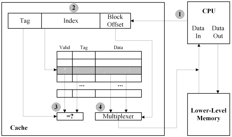
The process starts with the CPU sending an address to the cache (1). The cache splits this address into three components (2). The block offset component is used to index into a cache line, since each cache line can contain more than one CPU word. The index component is used to select a particular associative set in the cache. Hence the range of the index field, in binary, matches the number of associative sets in the cache. If the cache is direct mapped then the index component of the address has an address space just large enough to individually identify every line in the cache. The tag component is composed of whatever is left of the CPU address after the block offset and index components have been removed. The tag is used to distinguish between items in the set of potential main memory data, with the same index field, that can be stored in the same cache line.
Lastly, the cache examines the valid bit and tag entry for the cache line(s) specified by the index field of the CPU address (3). If a cache line's valid bit is set, and the tag entry from the cache matches the tag in the CPU address, then a cache hit has occurred. The required CPU word is extracted from the relevant cache line data block by indexed the block with the block offset component of the CPU address (4).
The reason behind using a CPU cache is the principle of locality, which is described below:
The property of locality has two aspects, temporal and spatial. Over short periods of time, a program distributes its memory references non-uniformly over its address space, and which portions of the address space are favoured remain largely the same for long periods of time.
This first property, called temporal locality, or locality by time, means that the information which will be in use in the near future is likely to be in use already. This type of behaviour can be expected from program-loops in which both data and instructions are re-used.
The second property, spatial locality, means that portions of the address space which are in use generally consist of a fairly small number of individual contiguous segments of that address space. Locality by space, then, means that the loci of reference of the program in the near future are likely to be near the current loci of reference. This type of behaviour can be expected from common knowledge of programs: related data items (variables, arrays) are usually stored together, and instructions are mostly executed sequentially.
Since the cache memory buffer segments of information that have been recently accessed, the property of locality implies that needed information is also likely to be found in the cache.
As an example of how the cache
utilisation is calculated, consider a direct-mapped cache with ten lines that
services one hundred trace file references, each of which requires a new block
to be loaded from main memory. If
each cache line is loaded with a new block ten times during the simulation then
the cache utilisation will be 100% as the loads to the cache are evenly
distributed. However, if just one
cache line was loaded with a new block one hundred times then the cache
utilisation would be 10% as just one cache line receives the entire load.
Whilst the above example is theoretically possible, in practice calculating the cache utilisation is more complex. An additional factor to be taken into account when calculating the cache utilisation is the replacement policy. Whilst the LRU and random replacement policies have no effect on the simple algorithm outlined above, if the replacement policy is FIFO then, if the above method is used, it will always appear that the cache has low utilisation because only the first line of each associative set will ever be loaded with a new block. The solution to this problem is to treat each associative set as just one cache line for the purposes of calculating the cache utilisation. Hence the cache utilisation calculation for caches using a FIFO replacement policy indicates the distribution of block-loads between the different associative sets, as opposed to different cache lines. As a consequence, the utilisation for a FIFO fully associative cache is always 100%.
The formula used to calculate
cache utilisation for a direct mapped cache in HASE Dinero is shown below:
sum = 0;
avg = (Number_of_Trace_References/Number_of_Cache_Lines);
for(i=0;
i<Number_of_Cache_Lines; ++i){
if((Number_of_Block_Loads[Line_i]-avg)<=0){
sum += Number_of_Block_Loads[i];
}
else sum += avg;
}
return((sum/Number_of_Trace_References)*100));
The Miss Breakdown is divided into three categories in HASE Dinero. The
method of calculation for each miss type is shown below:
|
Compulsory cache misses are regarded as all misses to the cache that are loaded to a cache line which has not yet had its valid bit set. |
|
|
Conflict cache misses are caused by any miss that occurs after every line in the cache has had its valid bit set. |
|
|
Capacity
misses are caused by any miss that both occurs before every line in the
cache has its valid bit set, and also causes valid cache data to be
overwritten. |
An
unfortunate side-effect of the low-overhead implementation of the miss breakdown
scheme employed is that once the cache is full no more compulsory or conflict
misses can occur. As a consequence,
in order to gain observable ratios in the miss breakdown the number of trace
file references processed must be limited to a number proportional to the number
of lines in the cache being simulated. Whilst
this number can be arbitrarily chosen, I recommend processing 150 trace file
lines for each cache line. Note
that as long as the same number of trace file lines are processed for each cache
line, the miss breakdowns of any cache configurations with the same number of
cache lines can be compared.
If
a comparison of the miss breakdown between cache configurations with a varying
number of cache lines is to be performed then the number of trace file
references processed should remain constant.
I have found that setting the number of input trace file lines to be
processed to 150 for each cache line in the cache with the largest number of
cache lines provides characteristic miss breakdown ratios as the cache size and
block size vary.
![]()