Thomas Zurek
Department of Computer Science
University of Edinburgh
Scotland / UK
Email: tz@dcs.ed.ac.uk
| Published in: | "Datenbanksysteme in Büro, Technik und Wissenschaft", Proc. of the BTW'97 (German Database) Conference, Ulm, Germany, March 1997 |
| Publisher: | Springer Verlag, GI Informatik aktuell |
| Pages: | 269 - 278 |
Abstract: We present a framework for parallel temporal joins. The temporal join is a key operator for temporal processing. Efficient implementations are required in order to make temporal database features attractive and applicable for the many applications that are amenable.
We focus on the temporal intersection as the supertype of temporal joins. In contrast to traditional equi-joins, parallel temporal join processing suffers from tuples being replicated between data fragments. This causes a significant overhead.
A basic parallel temporal join strategy - derived from traditional approaches - is refined by two optimisations. The quantitative impacts of the optimisations are evaluated. It is shown that both optimisations together decrease the basic costs significantly.
Keywords: temporal join, temporal databases, parallel databases, data partitioning.
The temporal join is one of the key temporal relational operators. Intuitively, it is used whenever we want to retrieve data that is valid at the same time. Efficient implementations are required in order to make temporal database features attractive and applicable for the many applications that are amenable to temporal data processing. The performance of temporal join processing, however, suffers from the higher size of temporal relations because tuples are logically deleted rather than physically removed, and from the high selectivity factor of temporal join conditions.
Various authors argue that the semantics of time can be used for optimisations. A popular example is the `append-only' characteristic of transaction time applications: when new tuples are inserted they are appended to the collection of existing ones. This results in a natural sort order on the transaction time attribute. The sort order itself can then be exploited in several ways.
Parallelism is another possibility of improving temporal processing performance. It has already been successfully incorporated in traditional database technology and helped to overcome certain performance deficits. However, it has been widely neglected in the context of temporal databases. To our knowledge, there has been only one paper that discusses parallel temporal issues [9]. Its optimisations, however, are bound to special cases of temporal joins and there is no quantitative evaluation.
In this paper, we want to overcome some of these deficits and present a framework for parallel temporal join processing. We thereby concentrate on features that are temporal-specific; considerations on data skew or optimisations based on non-temporal parts of the join condition are left out as these have been discussed already by other papers and in more detail. Section 2 discusses types of temporal joins and sequential algorithms that were proposed in the past. Section 3 shows a simple example that should make the reader aware of the temporal-specific problem of parallel join processing. In section 4, two optimisations for parallel temporal joins are presented. Section 5 evaluates these results quantitatively. Finally, the paper is summarised and concluded in section 6.
An interval [t_s,t_e] consists of a start point t_s and an end point t_e and includes all time points in between and including these. We adopt the most frequently used temporal data model in which each tuple holds an interval timestamp [7].
The literature has mainly concentrated on a `supertype' of the joins that arise from Allen's relationships, namely the temporal intersection that includes the relationships equals, overlaps, during, starts and finishes. We will focus on intersection joins as all the other temporal joins can be considered as intersection joins with additional constraints. Furthermore we can draw a clear line between the optimisations that are possible for the temporal intersection join and those that are specific to the other temporal joins.
Basic nested-loops for equi-joins usually perform badly because they test every tuple combination given by the cartesian product of the participating relations. Of these combinations only few qualify for the result. Other algorithms avoid this by partitioning the data prior to the joining stage. The sort-merge approach is based on implicit partitioning given by a sort order on a join attribute. The hash join approach requires explicit partitioning prior to its joining stage whereas index based joins use precomputed partitioning [11].
In the literature, several algorithms based on these approaches have also been discussed in the context of temporal joining. Sort orderings on the temporal attributes - these are either achieved through explicit sorting or implied by the `append-only' characteristic of transaction-time relations - allow various optimisations. Discussions can be found in [3], [8], [4], [12].
In the case of equi-joins, explicit partitioning is the basis for very efficient joining. Applying those techniques to temporal intersection of interval data, however, has the problem that intervals cannot be reduced to a discrete value that allows the grouping of the tuples whose timestamps intersect in one single partition. One way to get around this problem is to group tuples by either one of their temporal interval boundaries (start or end point) or a combination of these (e.g. in [10]). Tuples must then be either replicated and put into those partition fragments that hold other tuples that possibly join, i.e. have intersecting timestamps (as in [9] and [13]) or each partition fragment has to be joined with various others that hold possibly joining tuples (as in [10]). The algorithm proposed in [13] processes fragments sequentially and keeps tuples that have to be present in the following fragment in a cache. This makes it an inherently sequential algorithm.
Replication cannot be avoided in the case of parallel temporal join processing. Such an approach is discussed in [9]. The so called asymmetry property of relations - that appears e.g. in contain- or overlap-joins - can be used for reducing the number of tuples that have to be replicated. Asymmetry, however, does not occur in the more general intersection join. Therefore, most optimisations that are suggested by Leung and Muntz cannot be applied in the case of the intersection join.
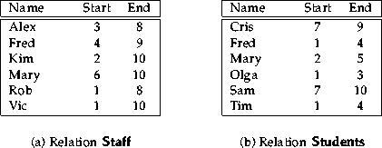
Figure 1: An example of two temporal relations.
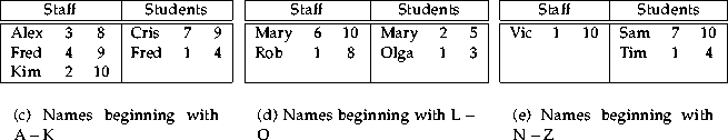
Assuming that the names are unique we can get all persons who studied and worked in the department by computing an equi-join R ¤ S with the join condition C = (Staff.Name = Students.Name). To compute this join in parallel we can partition the two tables by using the values of the name attributes. Figure 2 shows an example for partitioning the tables into three fragments respectively and thus into three smaller and independent joins. Please note that the partitioning process produced disjoint fragments respectively. Each of the three joins can be processed on different nodes in parallel.
Figure 2: Example of processing an equi-join in parallel.
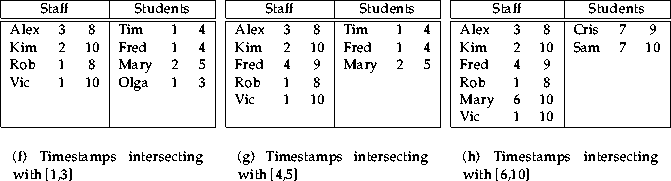
If we want to relate staff members and students who worked and studied at the same time in the department then we need a temporal intersection join between the two relations. The join condition is C = (TIMESTAMP(Staff) = TIMESTAMP(Students)) in this case. Similarly to the equi-join above, the temporal join can be processed in parallel. This time, however, the tables have to be partitioned over the interval timestamps. Figure 3 shows an example of partitioning the tables into three fragments respectively. Please note that the fragments are not disjoint in this case and tuples are replicated. This causes an overhead not only because of the effort spent on the replication itself but also because of the additional work imposed on the joining of the fragments.
Figure 3: Example of processing a temporal join in parallel
where the Rk and Sk are referred to as fragments of R and S respectively. There are several ways for creating the Rk and Sk: section 3 showed an example of range-partitioning, i.e. the partition attribute's domain is divided into several ranges and a tuple is placed into the fragment that corresponds to the range that its partition attribute's value falls in. In the case of an atomic attribute domain, this is just a special type of hash-partitioning where a hash function is used to assign a tuple to a fragment. This naturally leads to disjoint fragments as there is only one hash value for each attribute value.
Hash partitioning, however, does not work for interval data: assume that there was a hash function f such that intersecting intervals are assigned to the same fragment with at least two different fragments to be created. Let [x_s,x_e] and [y_s,y_e] be two non-intersecting intervals, i.e. x_s <= x_e < y_s <= y_e, assigned to two different fragments i and j by f, i.e.
Now consider the interval [x_e,y_s] which should fall into fragment i because it intersects with [x_s,x_e] but also into fragment j because it intersects with [y_s,y_e]. Thus f would have to assign two different values i and j for [x_e,y_s] which contradicts its notion of being a function. Thus, in general, it is impossible to create disjoint fragments for interval data and it is necessary to replicate tuples. In sections 4.2 and 4.3 two measures are presented to reduce the overhead imposed by tuple replication.
For that purpose, we can divide a fragment Rk into two subfragments R'k and R''k. R'k holds the tuples whose timestamp startpoint falls into the k-th range - these are called the primary tuples - and R''k holds tuples that are already in some fragment Rj with j<k - these are called the replicated tuples. A partial join then looks like this
However, the join R''k ¤ S''k comprises exactly those `unnecessary' tuple joins that we have identified above. Processing can therefore be restricted to the first three joins in (2).
One might argue that optimal join ordering and avoiding I/O accesses by optimally using main memory is no special feature of temporal join processing. However, there are two significant issues about this second optimisation:
On a uniform workload[+], three different joins strategies were tested: Join A: traditional approach as in (1), Join B: join A plus optimisation 1, Join C: join A plus optimisations 1 and 2. We compared the performance of the three joins varying the number N of processing nodes. Figure 4 shows the result. As it can be expected join C performs better than join B which itself is better than join A. Interesting facts, however, are the quantitative effects of the optimisations: Optimisation 1 (join A -> join B) improves performance by between 20% (N=10) and 65% (N=50); Optimisation 2 (join B -> join C) decreases costs by 90%; Optimisations 1 and 2 (join A -> join C) give a composite improvement of around 95%. The experiments showed that the costs are dominated by the costs for the partial joins; partitioning costs and therefore communication costs can almost be neglected. The costs of joins A and B mainly comprise I/O costs whereas join C's costs consist of CPU and memory access costs. Increasing N implies a higher total I/O bandwidth, more memory and more CPU power. This explains the ideal speedup in figure 4.
Figure 5 shows the split of costs for join C. Graphs for the other two joins look the same; only the respective cost values on the vertical axis are higher but the ratio between the partial cost components is the same. The replication join costs are the costs for performing the joins that are due to tuple replication, i.e. the joins involving R''k and S''k. The primary join costs are the costs for performing the join R'k ¤ S'k.
The overhead costs imposed by tuple replication have a share of 65% to 75% of the total costs. This suggests that any optimisations that reduce tuple replication should translate nicely into a total cost reduction.
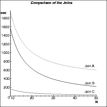
Figure 4: Performances of the three join strategies
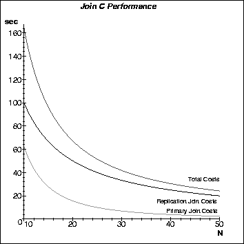
Figure 5: The components of the join C costs
Parallelising temporal joins is not trivial. The significant difference with respect to traditional equi-joins is based on the fact that timestamps are usually represented as intervals. The intersection conditions consist of non-equality predicates. Data partitioning over time intervals is therefore not straightforward: tuples have to be replicated and to be put into several fragments of a range-partition of the temporal relations. This causes a considerable overhead.
We showed that this overhead can be reduced significantly if one divides a data fragment into primary and replicated\ tuples. This allows to avoid that replicated tuples of one relation are joined with replicated tuples of another relation as this is not necessary (optimisation 1). Furthermore this division enables us to choose a certain number m of fragments such that subfragments that contain the primary tuples fit into main memory. This allows to reduce I/O accesses significantly (optimisation 2).
Finally, the effects of the optimisations were evaluated quantitatively. Both optimisations reduced costs by around 95%. A further conclusion was that the overhead caused by tuple replication made up around 70% of the total costs. Research efforts on reduction of tuple replication should therefore translate nicely into performance improvement.
An open issue is the choice of an appropriate partition for the temporal relations. This choice is very delicate as it has to cope with data skew and also determines the rate of replication. We plan to investigate this problem in the near future.
This document was generated using the LaTeX2HTML translator Version 96.1 (Feb 5, 1996) Copyright © 1993, 1994, 1995, 1996, Nikos Drakos, Computer Based Learning Unit, University of Leeds.
The command line arguments were:
latex2html -split 0 -t T. Zurek: Parallel Temporal Joins -address Thomas Zurek, tz@dcs.ed.ac.uk -ascii_mode -show_section_numbers tj.
The translation was initiated by Thomas Zurek on Tue Mar 11 11:35:20 GMT 1997