Hash Joins

The performance gain achieved by the sort-merge join is based on the facts that during the sorting stage

For an equi-join the sort-merge algorithm only exploits (1). This suggests that sorting the relations is actually too much; methods that create a situation as described by (1) are sufficient.

Hashing the relations is such a method. It creates a set of hash buckets with each bucket being associated either with one join attribute value or a range or set of such values. A hash function h that takes a join attribute value as an argument then assigns a tuple to a bucket. Consider, for example, the following join that was discussed in section 3.2:

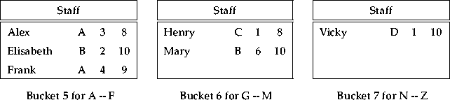
$\begin{displaymath} \text{\tt Staff} \;\Join_{\scriptscriptstyle C}\; \text{\tt Student}\end{displaymath}$

with $C \;\equiv\; \text{\tt Staff.Name} = \text{\tt Student.Name}$

We can hash the relation Staff on the join attribute Name using a hash function that assigns the tuples to three buckets. Each bucket is supposed to hold tuples according to the letter with which the Name value starts. See figure 3.10 for the result. Next, we can subsequently read tuples from Student. Using the same hash function, we can find out in which bucket those tuples of Staff are to be found that can match with the respective tuple of Student. 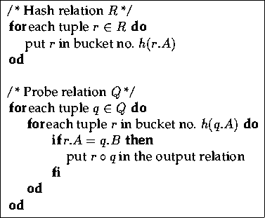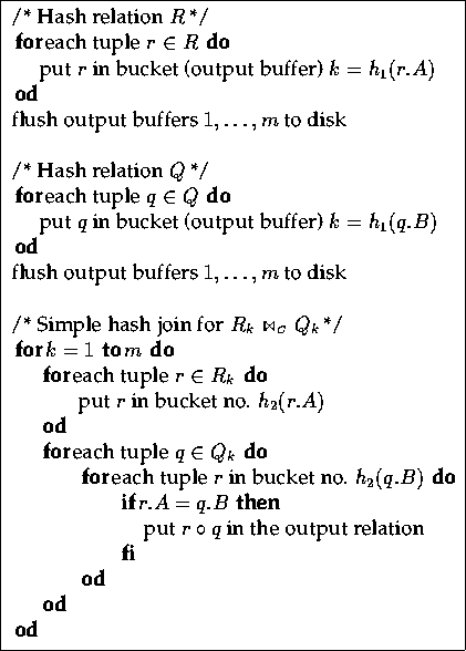Put the other way: all the tuples in the other buckets can be discarded; the actual join for a particular tuple can be concentrated on the tuples in a certain bucket. This algorithm is called the simple hash join [DeWitt and Gerber, 1985]. It is summarised in figure 3.11 for the case of an equi-join.

**Figure:** Example for hashing the relation `Staff` into buckets.
$\begin{figure} % latex2html id marker 1915 \begin{center} \begin{footnotesize} ... ... & \\ & & & \\ \hline\end{tabular}} }\end{footnotesize}\end{center}\end{figure}$

**Figure:** Simple hash join.
$\begin{figure} \begin{center} \fbox { \begin{minipage} {\textwidth} \begin{tabb... ...\ \\ gt {\bf od}\\ {\bf od}\end{tabbing}\end{minipage}} \end{center}\end{figure}$

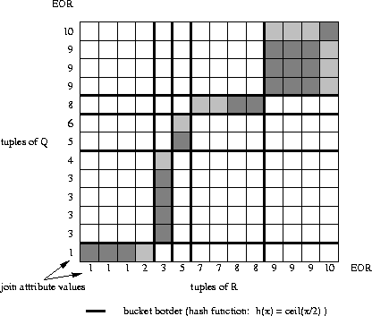
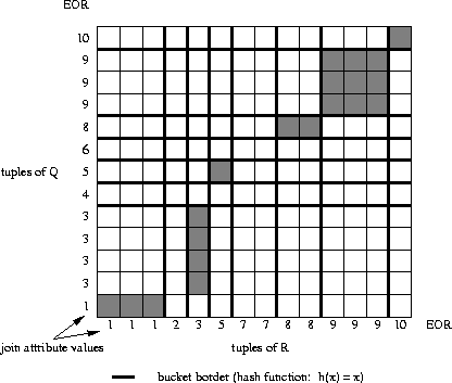
The search strategy for a simple hash join depends on the respective hash function that is employed. Figures 3.12 and 3.13 show two examples for the scenario that we have already used for analysing the nested-loop and sort-merge algorithms. In this case, the hash function divides the join attributes' domain into several ranges. In figure 3.12, for example, five ranges are created, each one associated with a bucket. The hash join algorithm then searches the `rectangles' that arise from corresponding buckets. This causes only a small number of mis-hits if the partitioning is not complete (figure 3.12) and none if it is (figure 3.13).

**Figure:** Search strategy of a simple hash equi-join.
$\begin{figure} \epsfxsize=0.9\textwidth \centerline{ \epsffile{/home/tz/work/thesis/fig/j-hash-1.ps}} \centerline{ } \end{figure}$

**Figure:** Search strategy of a simple hash equi-join with complete partitioning.
$\begin{figure} \epsfxsize=0.9\textwidth \centerline{ \epsffile{/home/tz/work/thesis/fig/j-hash-2.ps}} \centerline{ } \end{figure}$

Hash joins have several advantages. If the hash table , i.e. the set of all hash buckets, fits entirely into main memory, the hash join has to scan each relation only once. For that reason, it is usually the smaller of the two relations that is hashed in the beginning [Bratbergsengen, 1984]. The performance of the hash join depends on the quality of the hash function and its implications, such as the number of buckets or the value ranges that are assigned to the buckets. If there are only a few ranges then there might be a large number of unnecessary comparisons because each bucket has to hold a large number of tuples. Furthermore, data skew [Walton et al., 1991], i.e. non-uniformly distributed data, and an inadequate choice of value ranges can cause certain buckets to hold a large number of values whereas others might be empty. This can also lead to a large number of unnecessary comparisons.

A variation of the simple hash equi-join, as illustrated in figure 3.11, is the Grace hash equi-join which was proposed in [Kitsuregawa et al., 1984]. It precedes the simple hash join by an additional partitioning stage: first, relations R and Q are hashed into buckets $R_1, \dots, R_m$ and $Q_1, \dots Q_m$ using a hash function h₁. This creates a situation in which tuples of a bucket R_k can only join with tuples in Q_k. Thus the join $R \Join_{\scriptscriptstyle C}Q$ is divided into or partial joins $R_1 \Join_{\scriptscriptstyle C}Q_1$ ,..., $R_m \Join_{\scriptscriptstyle C}Q_m$ which are performed by a simple hash join each. See figure 3.14. Obviously, the Grace hash join method can be generalised allowing sort-merge or nested-loop techniques for processing the partial joins $R_k \Join_{\scriptscriptstyle C}Q_k$ .Furthermore, the computation of the partial joins can be concurrent . These aspects will be discussed in section 3.5.

**Figure:** Grace hash join.
$\begin{figure} \begin{center} \fbox { \begin{minipage} {\textwidth} \begin{tabb... ...\ \\ gt {\bf od}\\ {\bf od}\end{tabbing}\end{minipage}} \end{center}\end{figure}$

A further improvement of the Grace hash join was proposed in [DeWitt and Gerber, 1985] and [Shapiro, 1986]: instead of flushing tuples of R₁ to disk they are kept in memory and joined with tuples that are found to fall into Q₁ during the hashing stage. Thus the joining stage only deals with the joins $R_2 \Join_{\scriptscriptstyle C}Q_2$ ,..., $R_m \Join_{\scriptscriptstyle C}Q_m$ .

In general, hash-based joins have been found to be some of the most efficient join techniques [Gerber, 1986]. Problems arise in situations with heavily skewed data or for nonequi-joins. Hashing is not only useful to reduce the number of unnecessary comparisons but also allows the decomposition of one big join operation into several smaller and independent ones. This is especially important for the parallelisation of joins which is to be discussed in section 3.5.

In many situation, hashing has proved to be more efficient than sorting. The latter observation has motivated G. Graefe to publish a paper with the title Sort-Merge-Join: An Idea Whose Time Has(h) Passed? [Graefe, 1994] in which he analyses the duality of sort- and hash-based query processing. He concludes that the sort-merge approach (for equi-joins) is almost obsolete with very few exceptions.