Recent years have seen an increasing number of technological and economical developments that affect the way in which database systems are used. Data warehousing , data mining , geographical and other information systems, e.g. on the internet, have added new requirements with respect to data modeling and processing performance. As a consequence, many new complex data types, such as spatial, temporal, audio and video data, have been introduced into database management system software. This process has been supported by technological progress, such as the advent of affordable, off-the-shelf parallel hardware which has been widely driven by the high demands of commercial database applications.
In this development, the relational data model plays a key role: on the one hand, it can be relatively easily enhanced to provide the new data types and, on the other hand, it provides a lot of opportunities to exploit new technology, in particular parallelism. The key to the success of parallelism in database technology is that it is largely invisible to the end user and database applications programmer. The team in the database management system vendor's research and development lab provides the basic, general-purpose techniques and the local database administrator fine-tunes the systems, based on characteristics of the local installation's data. The key issue in the way temporal data is introduced is that this present arrangement of hiding parallelism is continued.
In this thesis, we want to contribute to building the connection
between new data types and new technology. We will look at the
possibility of how time interval data can be joined in
parallel by partitioning the time interval data over several
processing nodes. Data partitioning is a key
issue in parallel database systems. I/O parallelism , for example, is based on physically partitioning data
over a large number of disks. This overcomes the ever increasing gap
between CPU speed and I/O bandwidth ![[*]](foot_motif.gif) . On
the processing side, data partitioning provides the opportunity to
magnify the raw computing power of individual commodity processors by
partitioning a workload into several portions which can be processed
concurrently.
. On
the processing side, data partitioning provides the opportunity to
magnify the raw computing power of individual commodity processors by
partitioning a workload into several portions which can be processed
concurrently.
However, data partitioning is not only beneficial for parallel but for
sequential join processing. In many situations, it also reduces the
amount of processing that is necessary to complete the task. In the
case of join processing, for example, we can separate tuples that
cannot possibly join by partitioning the data over the join attribute
values. Therefore, data
partitioning provides advantages in a parallel and a sequential
environment. We pay attention to this fact by looking at
partitioned temporal join processing, thus considering data
partitioning in a wider context although parallelism will be the main
focus.
Furthermore, we stress that our work is not restricted to time intervals but applies to interval data in general. However, interval data is mainly used in the context of temporal database applications and we can derive many requirements and constraints by looking at temporal scenarios. Therefore, we will focus on time intervals.
Before digging deeper into partitioned temporal join processing we want to illustrate some of the temporal- and interval-specific problems by an example.
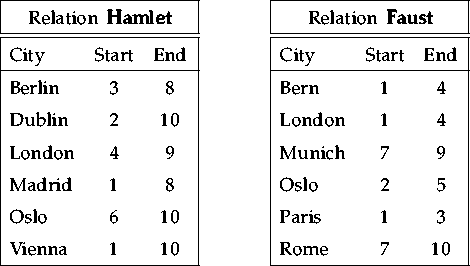
For this purpose, the two simple temporal relations of figure 1.1 are used: one holds cities and periods during which the play `Hamlet' is performed in the respective city, the other does the same for the play `Faust'. For simplicity, we use integers to denote dates.
If we want to find the cities in which both plays are performed then we can do this by computing the join
![]()
![]()
If we want to find those periods during which both plays are performed, irrespective of the location of the performances, then we need a temporal intersection join between the two relations. The join condition is
![]()
The problem of intervals overlapping partition breakpoints not only makes it difficult to choose appropriate breakpoints but also makes it delicate to determine the number of breakpoints: in order to reduce the number of overlaps one has to reduce the number of breakpoints but in order to increase the number of partial joins - e.g. in order to increase the degree of parallelism - one has to increase the number of breakpoints. Thus there are two contrary effects associated with interval partitioning; note that the first one does not exist in the case of an equi-join. This indicates that it is not straightforward to find the optimal trade-off partition between minimal overlaps and maximal parallelism. Apart from that, one has to expect further cost constraint given by the actual hardware platform and the join algorithm.