Spatially Partitioned Temporal Join

In this section, we describe a partition scheme which was proposed by [Lu et al., 1994]. It creates disjoint fragments for both relations. Hence, it is a symmetric partitioning approach. On the other side however, a fragment of one relation needs to be joined not only with one fragment of the other but - depending on its index number - with a set of fragments. Thus, if this method is to be parallelised, fragments need to be replicated in order to achieve independent partial joins. From this point of view, one could also speak of a fragment-and-replicate approach.

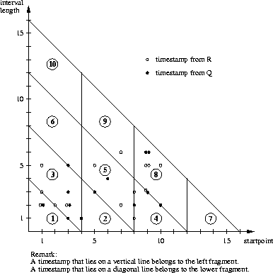
Lu et al. use a spatial rendition which was described in [Hinrichs and Nievergelt, 1983]. An interval [t_s,t_e] is mapped to a point in a two-dimensional grid. Its coordinates, x and y, are calculated by the equations:

For processing the join $R \Join_{\scriptscriptstyle C}Q$ , a fragment R_k of R has to be joined with a certain set of fragments of Q. The members of this set are determined by k. The latter describes the position of the corresponding fragmentation area on the grid. This position indicates certain characteristics: for example, fragments that are positioned in the upper part of the grid hold tuples whose interval timestamp is quite long. These tuples are likely to join with many others. In contrast, short-lived tuples are situated in the lower part of the grid. These are likely to join with only a few tuples. Intuitively, this means that fragments in the upper part need to be joined with more fragments than those located in the lower part of the grid. For the situation in figure 4.13 the necessary combination of fragments is shown in figure 4.14(a). For a more formal description of how to calculate these combinations see [Lu et al., 1994]. The example of figure 4.13, however, has several empty fragments which reduces its matrix of necessary joins to the one shown in figure 4.14(b).

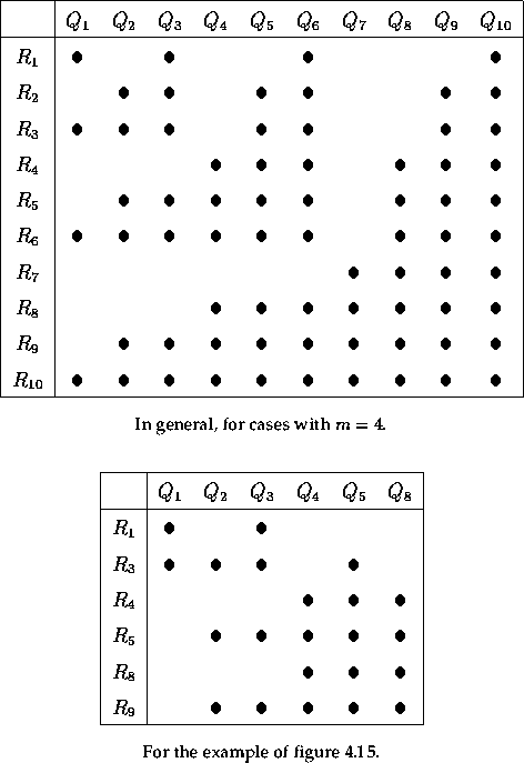
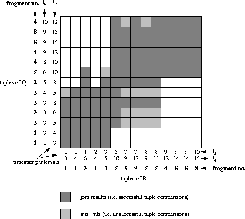
Figure 4.15 shows the resulting search strategy. It is quite efficient in avoiding unnecessary comparisons in this case. This, however, is partially due to the fact that the example has only a few long-lived tuples which causes fragments R₆, Q₆, R₇, Q₇, Q₉, R₁₀, Q₁₀ to be empty. These are all fragments which are usually involved in many partial joins (see figure 4.14(a)). This reduces the number of necessary partial joins significantly (see figure 4.14(b)). Furthermore we note that tuples from one relation may be loaded sequentially but tuples from the second relation might require several accesses.

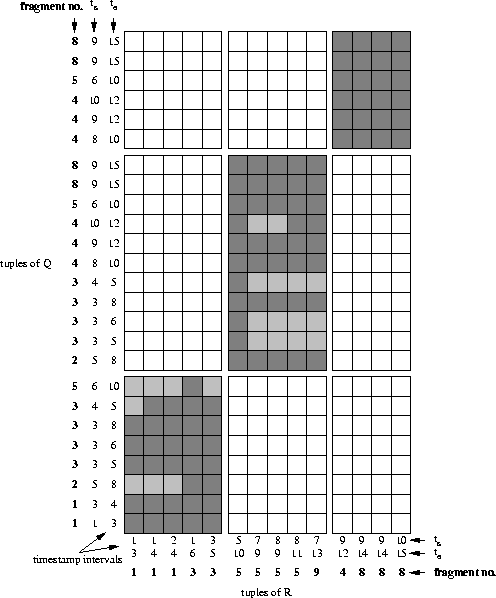
Alternatively, the partial joins can be processed in parallel. This, however, requires tuples of one relation to be replicated. Assume that this relation is Q. Consider now the example that we have used throughout the chapter. Regarding the matrix in figure 4.14(b) we note that R₅ and R₉ are to be joined with the same set of fragments of Q, namely Q₂, Q₃, Q₄, Q₅, Q₈. Thus we can pack R₅ and R₉ together into one `super-fragment' which is to be joined with those fragments of Q. This avoids the need to provide both R₅ and R₉ with a copy each of those fragments, thus reducing tuple replication. Similarly, R₄ and R₈ can be packed together. Even R₁ and R₃ can form a super-fragment as R₁ has to join with a subset of R₃'s Q-fragments. This groups the partial joins of figure 4.14(b) into three `super-partial joins'. This is illustrated in figure 4.16.

A major problem arises in the case that three or more relations participate in the join. Then, the structures depicted as matrices in figure 4.14 would have to be cubic or of higher order. This means that a huge number of fragment combinations have to be joined in order to compute the global result. For m=4, for example, there are 70 partial joins for a global two-way join (see matrix in figure 4.14(a)). For m=4 and a three-way join, however, there are already 528 partial joins to be computed.

The approach taken by Lu et al. is similar to many that have been used in the area of spatial join processing. Many spatial join algorithms are based on transforming an approximation of a spatial object into another domain, and performing filtering (e.g. in the form of partitioning) in the new domain [Patel and DeWitt, 1996]. Examples for such algorithms can be found in [Orenstein, 1986], [Orenstein and Manola, 1988] or [Becker et al., 1993].

**Figure:** Spatial rendition and numbering of fragments for the example.
$\begin{figure} \epsfxsize=0.9\textwidth \centerline{ \epsffile{/home/tz/work/thesis/fig/spatial-rendition.ps}} \centerline{ } \end{figure}$

**Figure:** Partial joins that are to be computed for processing the spatially partitioned join.
$\begin{figure} % latex2html id marker 4018 \begin{center} \mbox{ \subfigure[In ... ...e $\bullet$}& {\large $\bullet$}\\ \hline\end{tabular}}}\end{center}\end{figure}$

**Figure:** Search strategy for the spatially partitioned temporal join being processed sequentially. Partial joins are processed as nested loops.
$\begin{figure} \epsfxsize=0.9\textwidth \centerline{ \epsffile{/home/tz/work/thesis/fig/tj-spatial.ps}} \centerline{ } \end{figure}$

**Figure:** Search strategy for the spatially partitioned temporal join being processed in parallel. Partial joins are processed as nested loops.
$\begin{figure} \epsfxsize=0.9\textwidth \centerline{ \epsffile{/home/tz/work/thesis/fig/tj-sp-par.ps}} \centerline{ } \end{figure}$