Running without exploiting commutativity

The above example was run, but without specifying the functions a,b as commuting. This does not affect the value of the computation of f(8), but it does involve more computation, a 2069 node call graph this time. This is potentially 22% more computation than before.

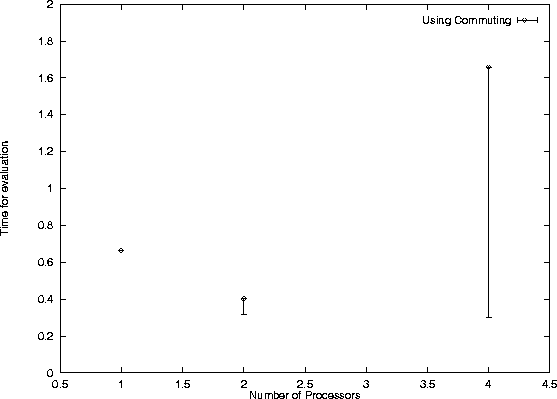
The advantage now is that there is now more parallelism in the evaluation, and therefore, if we run on more processors we can achieve a better speed up, and eventually will improve on the run time. I have also plotted the run-times for the one and two processor versions that exploit the redundancy, see fig. 7.3. This gives a cut off point at around 6 processors, assuming that we could run it on that number. This gives the result that by exploiting redundancy we can run the evaluation faster on 2 processors than on 4 processors without. Unfortunately, we cannot improve on this as we are limited by the parallelism in the function.

 

Figure 7.2:   Exploiting commutativity with different numbers of processors

 

Figure 7.3:   Comparison of exploiting / not exploiting commutativity

We return briefly to the analysis included earlier to see if the predictions for the size of these graph is borne out in practice. Recall the formula on page . For n=8, this gives a value of 1.58. If we compare this with the experimental result for this example of 1.23. The reason for the slight discrepancy is the fact that the example tree is not balanced, indeed at some points it is of depth 4, and at others depth 8. The formula implies that the deeper parts of the tree will have a greater proportion of redundancy, so the actual value is lower.