Nested-Loop Temporal Joins

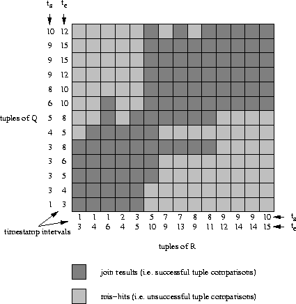
The basic nested-loop join, as outlined in figure 3.6, does not need to be adapted for processing temporal join conditions. It checks every tuple pair of the cartesian product anyway. Figure 4.2 shows an example of a temporal intersection join between two relations which are equal in size to the ones used in the example in chapter 3. The figure indicates that more tuple comparisons are successful than in the case of a nested-loop equi-join with equally sized relations. The nature of temporal join condition means that temporal joins (and especially temporal intersection joins) may frequently produce much higher join selectivities than comparable equi-joins. This means that an exhaustive search performed by a nested-loop join algorithm is possibly not as adverse as in the case of an equi-join.

The selectivities resulting from the temporal join condition considered here are more likely to lead to situations in which even small inputs can produce huge results. Such huge results are impractical to handle in both cases, as an end result but also as an intermediate result. An optimiser will therefore try to avoid to compute such gigantic joins either by warning the user about a possible huge end result (the user can then change or dismiss the query) or by rearranging the sequence in which the query operations are processed (such that a huge intermediate join result can be by-passed).

It is almost impossible to say what typical temporal join selectivities are. This is (a) due to the variety of temporal join conditions (see tables 4.1 and 4.2, for example) and (b) due to the great variety in the statistical characteristics of temporal applications which makes it already impossible to determine a typical selectivity for a pure intersection condition. The latter, for example, would depend on the typical interval length (which can vary widely between different applications), whether interval startpoints are spread uniformly over the lifespan (e.g. phone calls over a day) or whether they come in clusters (e.g. hourly measurements of certain parameters) and also the granularity of the time dimension.

  

Figure: Search strategy for a nested-loop temporal intersection join.