 |
The actual shape of the sort-merge join algorithm depends on the underlying join condition. In section 3.4.2, we outline the sort-merge join algorithm for an equi-join condition. For a temporal join condition, such as temporal intersection, the general structure remains the same: a sorting stage is followed by a merging stage. The merging stage, however, needs to be modified.
Most of the algorithms that have been proposed for temporal join processing employ a sort-merge strategy. Examples can be found in [Gunadhi and Segev, 1990], [Leung and Muntz, 1990], [Gunadhi and Segev, 1991], [Rana and Fotouhi, 1993] and [Segev, 1993]. Many authors consider their algorithms as refinements of the nested-loop approach that take advantage of the fact that one or all relations are sorted in ascending or descending order. This means that they merely discuss the merging stage of the sort-merge approach and assume that the required sort order is either enforced by a preceding sorting stage or already exists. The merging stage, however, can be regarded as nested loops in which the inner loop takes advantage of information that was obtained during previous loops.
Assuming the relations to be sorted can be reasonable, especially in the case of transaction time relations. Here, tuple timestamps are created according to the time of the update (i.e. the transaction time) . If these tuples are appended to the end of the relation we get a natural sort order of the tuples. This is sometimes called the append-only characteristic of transaction time relations.
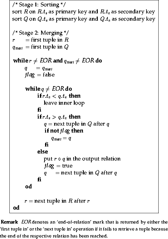
Figure 4.3 shows a sort-merge algorithm for a temporal intersection join. Originally, it was discussed as Algorithm 2 in [Rana and Fotouhi, 1993] which is similar to algorithm TJ-1 in [Gunadhi and Segev, 1991]. The two if-statements in the inner loop check the two situations in which no intersection occurs:
Figure 4.4 shows the search strategy of this algorithm. The outer loop moves along the horizontal axis whereas the inner loop scans vertically, along the column designated by the outer loop. Information obtained from previous loop runs provide a hint as to the best entry point in the column, i.e. several tuples at the beginning (coming from the bottom) might be omitted.