Overview

  In this section, we consider join techniques that include an explicit partitioning stage as an integral part of the join algorithm. They are shown in grey boxes in figure 4.7. In the case of the equi-join these techniques have proved to be very efficient and very versatile, especially allowing the parallelisation of the join operation. We might expect them to be similarly successful in the case of temporal joins.

  

Figure: Explicit partitioning joins.

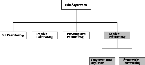We will merely concentrate on the symmetric partitioning  approach, i.e. both participating relations are partitioned; the fragment-and-replicate strategy  that was presented in section 3.5.1 is not affected by the actual join condition and therefore works in the same way for temporal joins as it does for any other type of join.

The basic temporal join strategy employing symmetric partitioning is built upon equation (3.6). It will be discussed in section 4.4.2. This will reveal the problem that the fragments R_k () cannot be disjoint because of the temporal intersection condition. This leads to certain negative implications:

1.

Replication Overhead:  During the partitioning process, a lot of tuples have to be (logically) replicated to be placed into several fragments. Please note that this logical replication   does not necessarily translate into a physical replication : when working on a shared-memory machine tuple fragments might be represented as an index, i.e. a set of pointers that refer to the actual locations in memory or on disk where the tuples are stored. In this case, the logical replication causes an additional effort when building these indices. When working on a shared-nothing architecture, however, logical replication is likely to be translated into a physical replication. In both cases, logical replication causes an overhead.  

2.

Processing Overhead:  Because of tuple replication, the individual fragments become larger. Hence, processing the partial joins requires more effort. This causes a processing overhead.  

3.

Duplicates Overhead:  Tuple replication can also produce duplicates in the result which either cause a further overhead in subsequent stages of a query evaluation or which have to be removed which itself is a potentially expensive process.  

• In section 4.4.2, a straightforward temporal adaption of the simple hash join is given. It suffers from all three overheads.
• In section 4.4.3, a join strategy is derived that reduces the processing overhead (b) and avoids the duplicates overhead (c). Effect (a), however, cannot be avoided when the partial joins have to be kept independent from each other for processing them in parallel. This strategy was originally proposed in [Zurek, 1996].
• In section 4.4.4, we present a strategy that was originally used in [Soo et al., 1994]. By sequentially processing the partial joins and keeping certain tuples in memory between each partial join evaluation one can avoid the replication overhead (a). Unfortunately, this method sacrifices the independence of the partial joins which therefore cannot be processed concurrently anymore.
• In section 4.4.5, a rather different approach is presented which is based on spatial partitions. It was proposed in [Lu et al., 1994] and maps intervals to points in a two dimensional space. This space is divided into disjoint parts which results in disjoint relation fragments. In this way, the replication and duplicates overheads , (a) and (c), are avoided. However, join processing requires a variable overlap of the fragments which either restricts the concurrency of the partial joins or requires fragments to be replicated, which means that the processing overhead (b) remains and a replication overhead might have to be re-introduced for parallelisation purposes.