The PEPA Eclipse Plug-in

A modelling, analysis and verification platform for PEPA

Adam Duguid, Stephen Gilmore, Michael Smith and Mirco Tribastone

Wednesday 01 December 2010

Abstract:
This user manual describes the PEPA Eclipse Plug-in, a modelling environment for the high-level modelling language Performance Evaluation Process Algebra, PEPA. The PEPA Eclipse Plug-in allows modellers to analyse their PEPA models using Markov chain theory, model-checking, and discrete or continuous simulation. The conversion from models in the PEPA process algebra to Markov chain models, simulation models, or differential equation models is entirely automatic. Analysis results are returned to the user in the form of graphs, charts and time series plots. A version of this document suitable for printing is available on-line.

6 Discrete and continuous simulation

1 Introduction

1.1 Getting Started

This guide provides a step by step description of the PEPA plugin.

It shows how you can edit PEPA models, carry out static analysis, obtain the underlying Continuous Time Markov Chain for steady-state analysis or perform time series analysis using Stochastic Simulation Algorithms or Ordinary Differential Equations. This guide will also describe how to use import/export tools for data exchange with third-party applications.

Familiarity with PEPA is assumed. To learn more about PEPA visit the PEPA web site.

1.2 The PEPA Perspective

The plugin provides an editor for PEPA model input files. The editor contributes a top-level menu item to the workbench bar through which all the PEPA-related tools are accessible. Additional information is provided via workbench views. The PEPA perspective provides a customisable layout for those views in the workbench.

To open the PEPA Perspective, select Window > Open Perspective > Other . Then select PEPA and press OK to finish.

2 Editing PEPA models

2.1 The PEPA Editor

The PEPA Editor lets you edit PEPA input model files. It is associated to open files with the .pepa extension in the workbench. In order for to open a PEPA input file in the Eclipse workbench, a project container has to be chosen.

To create a new project, select File > New > Project... . Then select General > Project . Choose a name and press Finish to complete.

To create a new file, right click the project and select File > New > File . Give the new file the extension .pepa

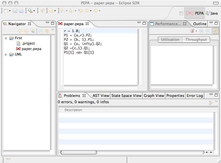
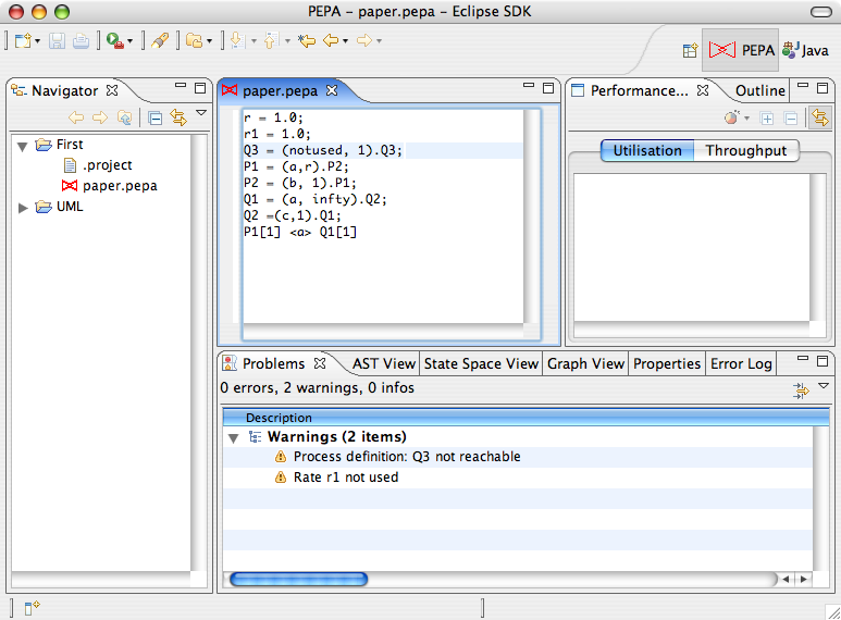
The input is parsed when the file is saved. If the parsing is successful static analysis is then carried out. Warning and errors generated by both the parser and the static analysis tool are shown in the Eclipse Properties View.

2.2 Basic Syntax

Rate Assignments must precede any process definition. A rate identifier is valid if it is a valid Java identifier starting with a lowercase letter. Rate assignments support expressions. They must end with a semicolon

                                r1 = 1.0;
                                r2 = 2.0 * r1 - 0.05;

Process Assignments A process identifier is valid if it is a valid Java identifier starting with an uppercase letter. As usual an identifier can represent a Choice or a Prefix. It can also identify subparts of the system when it is assigned a cooperation. Process assignments must end with a semicolon

                                P1 = (a, r1).P1 + (b, r2).P1;

Passive Rates can be specified as either infty or T. Weights can be assigned as integer numbers. Weights however cannot be rate identifiers. If no weight is specified, the default value 1 is assumed.

                                (a, T).P
                                (b, infty).P
                                (a, 3 * infty).P

Cooperation Sets are enclosed by . Cooperations with empty action set can be alternately specified with the parallel operation ||.

                                P <a,b,c> Q
                                P || P

Aggregation is partially supported by the plugin. If a cooperation on an empty action set between n is declared as P[n] then a canonical form representation for the process is considered during state space derivation of the underlying Markov chain.

3 Views

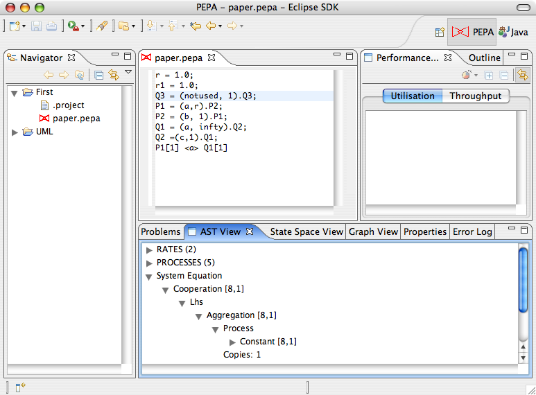
3.1 The Abstract Syntax Tree View

The AST View is a read-only Eclipse view for navigating the Abstract Syntax Tree of the model. The view is always associated to the currently active editor in the workbench.

3.2 Graph View

The Graph View is a tab-based view responsible for the management of all the graphs produced by the PEPA plugin. It is automatically opened when a new graph is requested. If you want to open it explicitely, select Window > Show View > Other... and then select PEPA > Graph View . The view support tools for editing graph properties such as background color, line thickness and legends. In addition, it provides a number of exporters to save the image to graphic formats such as PNG or serialise the data to file.

To edit the graph, right click it and select Properties... . To serialise the data, click the drop-down button in the toolbar menu of the view in the top-right corner of the view and select the desired format. A wizard will guide you through the process of setting exporter options and selecting target resources.

4 Markovian analysis

4.1 State Space Derivation

Once a model is successfully parsed, Markovian analysis can begin via state space derivation of the underlying Markov chain.

To derive the state space of the model in the active editor in the workbench, select PEPA > CTMC > Derive .

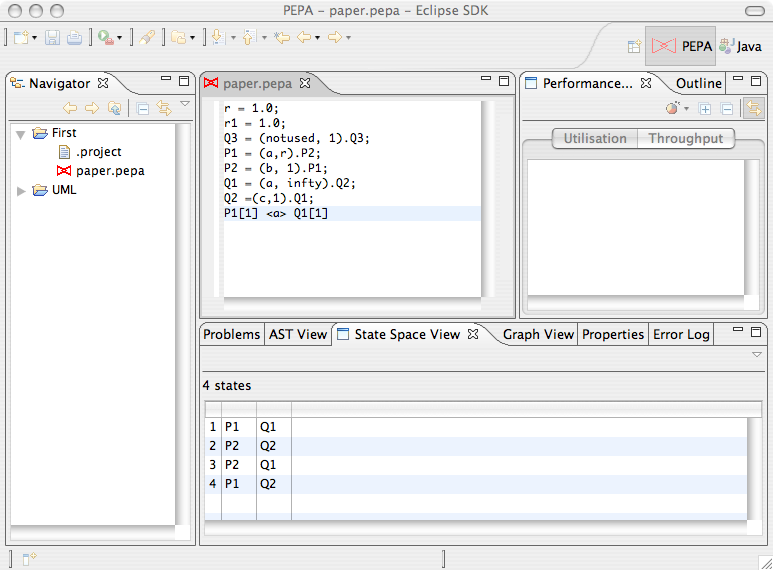
A tabular representation of the derived state space is shown in the State Space View

4.2 State Space View

The State Space View allows you to navigate the underlying CTMC of a PEPA model. After a model is derived, the view presents a tabular representation of the state space. The first column shows the state number, then there are as many columns as the number of top-level components. An additional column shows the steady-state probability of the state after the model is solved.

4.3 Filtering the State Space

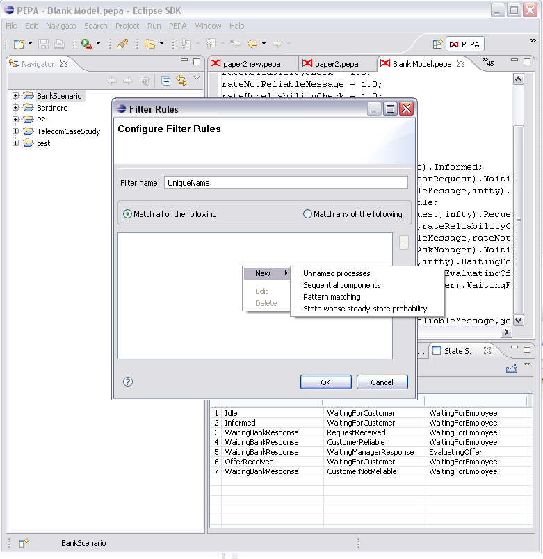
The view provides filters for the state space. Here are the filter rules available.

States with unnamed sequential components. States whose steady-state probability is in a given range. States matching a given pattern . States which have a top-level component in a given state. A number of rules can be grouped into a collection. The collection is assigned a name which is unique within the model's rule sets. You can specify any number of rule sets. However, only one rule set can be applied at a time. The rule setting are persistent across workbench sessions.

To open the filter rule editor, click the drop-down arrow in the State Space View toolbar.

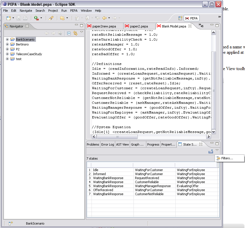
The State Space Filters dialog box will show the currently available filter sets for the model.

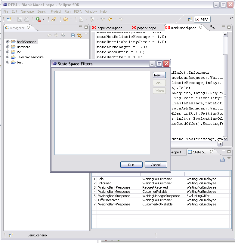
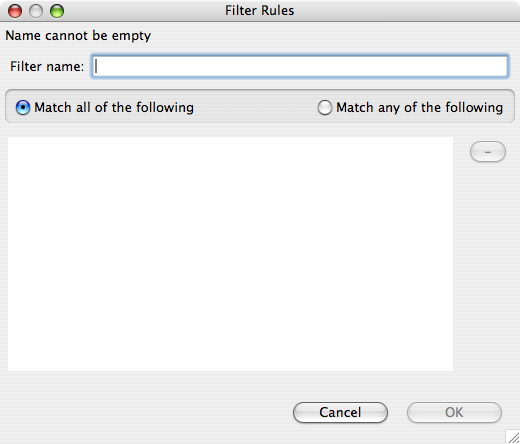
Click New... to edit a new set of rules. You are required to give it a name. The two radio buttons let you select between matching any or all of the defined rules. The rules are shown in the list box.

To manage the rule list, right click the list box. Click New to show the supported rules.

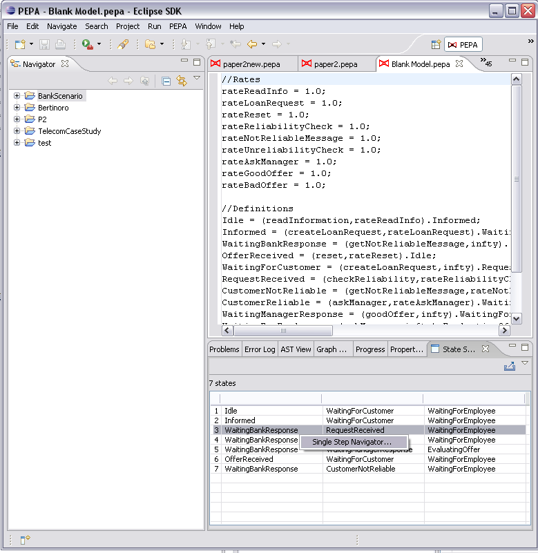
4.4 Single Step Navigator

The Single Step Navigator is tool for walking the state space graphically. It is particularly useful for debugging purposes. It consists of two tables containing the list of incoming and outgoing states. The sequential components which cause the transition to be performed are highlighted and an option allows you to make filtered states not walkable.

To open the navigator, right click a state in the state space view and select Single Step Navigator . The tool will be shown in a separate dialog box.

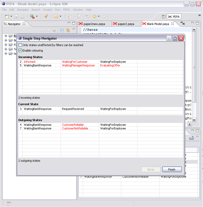
Double click a state to set the new current state in the navigator.

4.5 Exporting the State Space

The State Space View provides a wizard to export the state space into a csv (comma-separated values) files. To open the wizard, click the export button in the top right corner of the state space view.

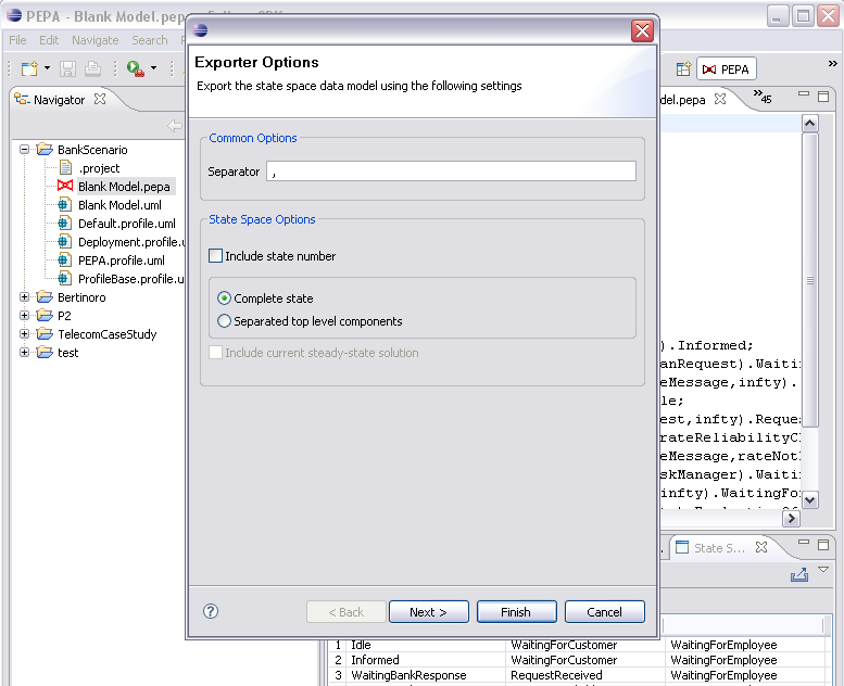
The wizard will produce two files, the generator matrix and the state space in the form of an ordered list of strings. The separator character will be used to delimit the values in the generator matrix files. If the Include state number option is checked, the state number will be prepended to state. The state can be represented fully or as an array of separated top level components. Moreover, if the steady-state solution is available, the steady state probability can be included in the state space file. The values of the state space files will be delimited using the separator character of the generator matrix.

Click Next to select the destination for the target files. The wizard doesn't allow to overwrite existing files.

4.6 Steady-State Analysis

To obtain the steady-state probability distribution of the underlying Markov chain of a PEPA model, click PEPA > CTMC > Steady State Analysis . The item is not be enabled if the state space is not derived.

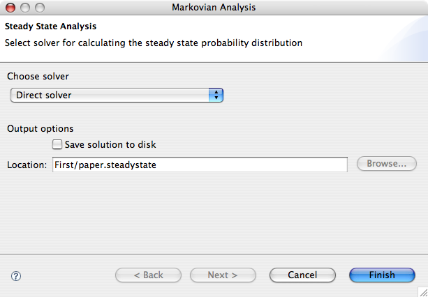
The wizard will guide you through the process of selecting a solver and setting its parameters. You can choose between a direct solver and a range of iterative solvers for which a number of preconditioners is available.

Once the model is solved, the State Space View will be updated with a column showing the steady-state probability of each column.

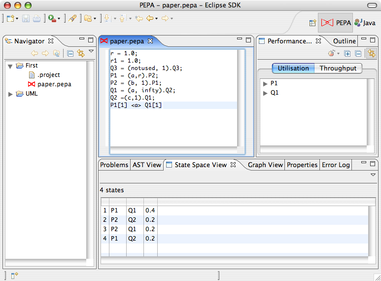
In addition, throughput and utilisation analysis will be carried out automatically and results will be available in the Performance Evaluation View.

5 Performance analysis

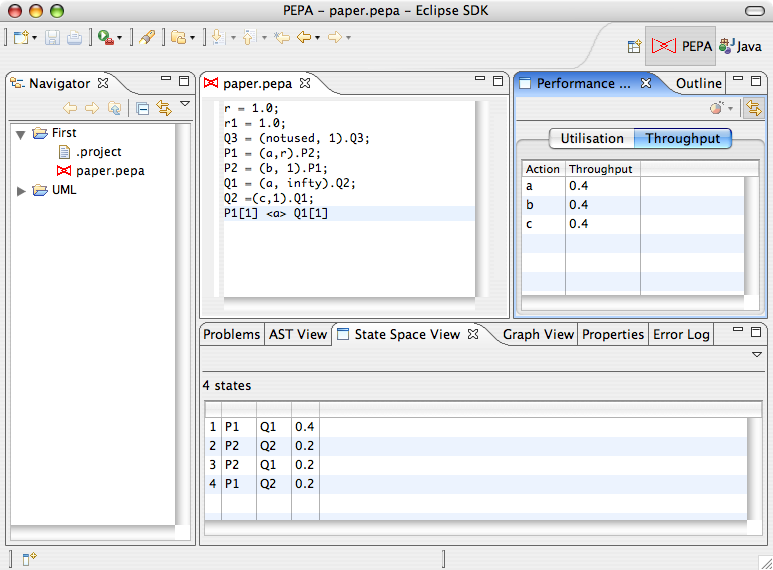
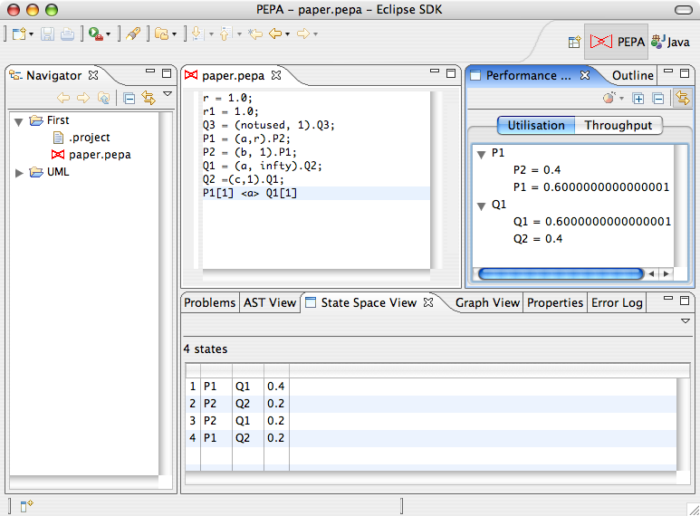
5.1 Performance Evaluation View

The Performance Evaluation View shows information about throughput and utilisation analysis. The view is automatically updated when the model in the active editor is solved.

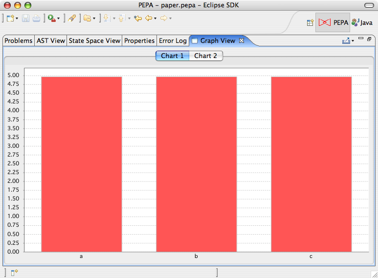
The Throughput Analysis tab lists the rate at which the actions of the PEPA model are performed at steady-state. A bar plot can be obtained by right-click the list and selecting Show graph . The corresponding graph will be shown in the Graph View.

The Utilisation Analysis tab is a tree-based view showing the long-run utilisation of each top-level component of the model. For each component, it shows the percentage of time it is in a particular local state. A pie chart of a component can be obtained by right-clicking the desired component in the tree and selecting Show graph . The corresponding graph will be shown in the Graph View.

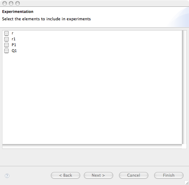
5.2 Experimentation

The plugin features support for experimentation, i.e. running a model with values for its parameters varying across desired ranges. The results of the experiment are plotted in the Graph View and a number of exporters is available for data serialisation.

To launch the experimentation wizard on the model of the active PEPA editor, select PEPA > CTMC > Experimentation...

The first page of the wizard lists the model parameters on which experimentation can be run. This will include the rate definitions as well as all the aggregation operators included in the model system equation.

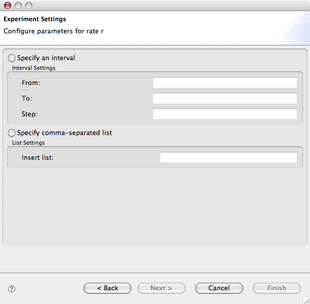
After Next is pressed, a wizard page for each selected parameter will let the user set the desidered range to be used in the experiments. Range can be specified in two different ways. For a uniform sampling over a given interval you may want to click the Specify an interval button. Otherwise, a comma separated list of values can be directly specified if the Specify comma-separated list is pressed.

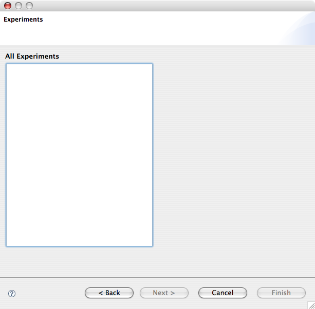
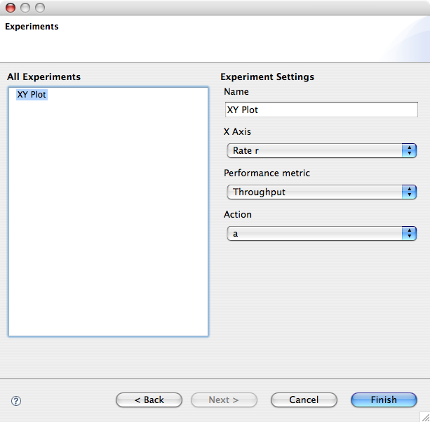
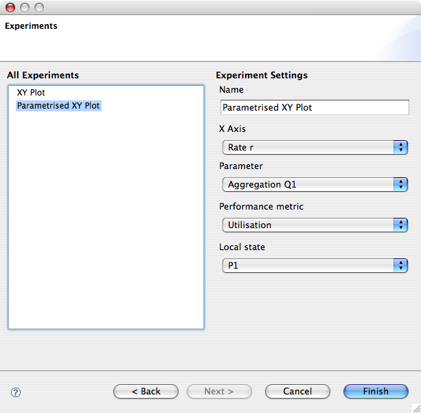
The last page of the wizard lets you create the experiments with the specified parameters. The plugin currently supports two types of experiments. A basic 2D graph plotting a performance metric against a parameter. A parametrised 2D graph plots a number of lines a performance metric against a parameter, a line for each value in the desired range of a second parameter.

The performance metrics available are: action throughput, sequential state utilisation, or steady-state probability of a subset of the state space as specified by a filter in the filter rule editor of the model.

To create a new experiment for a basic 2D graph, right click the list-box on the left of the wizard page and select New > XYPlot . The right hand side of the page will be dinamically updated with the widgetry for defining the experiment.

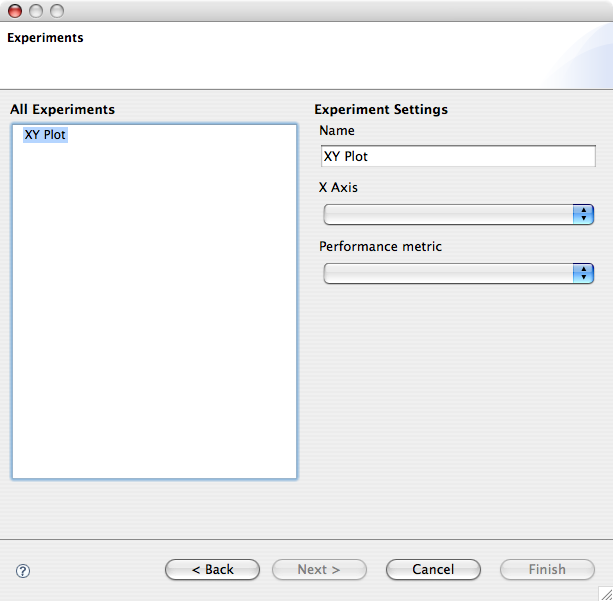
The name of the experiment will be shown as the title of the generated graph. The X Axis combo box lists the available model parameters and selection on the performance metric combo box will update the user interface with an additional section related to that performance metric. In the case of throughput, for example, a combo box lets the user select the action type.

To create a new experiment for a parametrised 2D graph, right click the list-box on the left of the wizard page and select New > Parametrised XYPlot . The user interface is very similar to that of the basic 2D graph, except for an additional combo box requiring the user to specify the second parameter.

To delete an experiment, right-click the experiment on the list box and select Delete

When you are done setting up the experiments, you can run them by pressing the Finish button of the wizard. The experiments will be run in the background and the results will be shown in the Graph View.