

Next: Partitioned Temporal Join for
Up: Explicit-Partitioning Join Algorithms
Previous: Simple Temporal Hash Join
Above, we identified successful but replicated tuple comparisons as a
major problem of the simple approach. A first measure could be to
extend the tuple comparisons by checking if the respective comparison
occurs somewhere else. This avoids duplicates in the result but does not avoid the actual unnecessary
tuple comparisons. Thus, it still produces a processing overhead.
Consequently, replicated tuple comparisons should be avoided all
together.
For that purpose, we observe the following: consider two tuples  and
and  with respective timestamps
[r.ts,r.te] and [q.ts,q.te]. Assume that the timestamps
intersect and therefore that r and q are compared with each other
at some stage of the computation. If r.ts falls in the i-th and
q.ts in the j-th range of the time domain then they are compared
in the partial join
  for the
first time. Possibly, they are compared again in subsequent partial
joins.
In order to avoid this, a fragment, say Rk, can be divided into two
disjoint subfragments, R'k and R''k. R'k holds
the tuples whose timestamp startpoint falls into the k-th range -
these are called the primary tuples - and
R''k holds tuples that are already in some fragment
Rj with j<k - these are called the replicated
tuples , i.e.
A partial join then looks like this
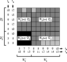
However, the join  comprises exactly those
unnecessary tuple comparisons that we have identified above;
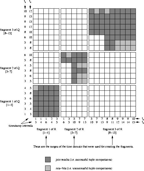
figure 4.9 illustrates this for the partial join
 of the example of figure 4.8.
Processing can therefore be restricted to the first three joins in
(4.2). We note that this restriction applies only
when the entire join
  is computed; for getting the result
of
  we still require
  because

if  and
and  . We note that
 due to the
definition of R''k and Q''k. In total,
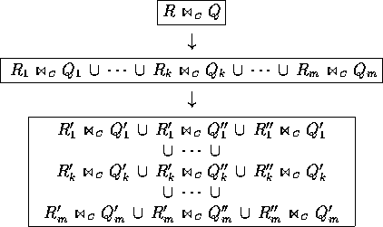
  can be
decomposed as shown in figure 4.10. This leads to
the search strategy shown in figure 4.11.
Figure:
Illustration of equation (4.2)
for  in figure 4.8.
 |
Figure:
Improved partitioning for computing a temporal intersection join.
 |
Figure:
Search strategy for the improved partitioned temporal join.
 |
A second optimisation is based on the following observation: if
the remaining three joins in (4.2) are processed
sequentially in one of the orders
- 1.
 or
or
- 2.

and R'k and Q'k fit, respectively, into the local main memory of
the processing node, then we can avoid unnecessary accesses to
secondary storage. We can, however, enforce this situation because the
sizes of the R'k and Q'k are much easier to predict and to
control than those of the R''k and Q''k (and consequently those
of Rk and Qk): each tuple of R and Q appears exactly in one
R'k and Q'k but might appear in several R''k or Q''k,
respectively. The assignment of a tuple to a certain R'k (Q'k
resp.) only depends on the value of the startpoint of the
timestamp . This, however, is nothing else than
partitioning atomic values as in the case of an equi-join. In the
simplest case, the number of fragments m can be chosen high enough
to fit the R'k and Q'k into main memory. More sophisticated
techniques might be necessary if the startpoint values are heavily
skewed , see e.g. [Hua and Lee, 1991] or [DeWitt et al., 1992].


Next: Partitioned Temporal Join for
Up: Explicit-Partitioning Join Algorithms
Previous: Simple Temporal Hash Join
Thomas Zurek
![]() and
and ![]() with respective timestamps
[r.ts,r.te] and [q.ts,q.te]. Assume that the timestamps
intersect and therefore that r and q are compared with each other
at some stage of the computation. If r.ts falls in the i-th and
q.ts in the j-th range of the time domain then they are compared
in the partial join
with respective timestamps
[r.ts,r.te] and [q.ts,q.te]. Assume that the timestamps
intersect and therefore that r and q are compared with each other
at some stage of the computation. If r.ts falls in the i-th and
q.ts in the j-th range of the time domain then they are compared
in the partial join ![]() for the
first time. Possibly, they are compared again in subsequent partial
joins.
for the
first time. Possibly, they are compared again in subsequent partial
joins.
![]()
 due to the
definition of R''k and Q''k. In total,