A more general, but also more delicate parallel joining technique is based on symmetric partitioning where all participating relations are partitioned. We have encountered this method already in the discussion of the Grace hash join (figure 3.14). Symmetric partitioning splits one `big' join into several smaller and independent ones:
| |
(9) |
The partial joins ![]() are
independent from each other and can therefore be processed
concurrently, i.e. in parallel. This parallelisation technique can
be applied to each join algorithm that was presented in
section 3.4. The Grace hash join in
figure 3.14, for example, can be considered as a
parallel hash join if the `for k=1 to m do' loop
is parallelised, i.e. if its body is executed concurrently.
are
independent from each other and can therefore be processed
concurrently, i.e. in parallel. This parallelisation technique can
be applied to each join algorithm that was presented in
section 3.4. The Grace hash join in
figure 3.14, for example, can be considered as a
parallel hash join if the `for k=1 to m do' loop
is parallelised, i.e. if its body is executed concurrently.
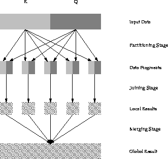
Figure 3.19 shows the structure of this family of parallel joins. It is divided into three stages:
 |
The parallelisation, motivated by (3.6), works
very well for equi-joins because it is easy to create
disjoint fragments ![]() (
(![]() respectively) which allow the partial joins to be independent.
Unfortunately, many nonequi-joins and - as we
will see in chapter 4 - many types of temporal joins
cannot be divided into disjoint fragments and maintain the
independence of the partial joins at the same time. One has then to
decide whether to sacrifice either the disjointness or the
independence with the first one being the preferable option in most
cases.
respectively) which allow the partial joins to be independent.
Unfortunately, many nonequi-joins and - as we
will see in chapter 4 - many types of temporal joins
cannot be divided into disjoint fragments and maintain the
independence of the partial joins at the same time. One has then to
decide whether to sacrifice either the disjointness or the
independence with the first one being the preferable option in most
cases.
The selectivities of the partial joins are much
higher than for the original join because the partitioning
concentrated tuples with similar values in associated fragments Rk
and Qk. This is an important point in the sense that the
selectivity is an important issue for the choice of the most
appropriate (sequential) join algorithm for computing the partial
joins ![]() . In a set of experiments that we conducted on
partitioned temporal joins, for example, we observed average
selectivities of 80% for the partial joins of a join
. In a set of experiments that we conducted on
partitioned temporal joins, for example, we observed average
selectivities of 80% for the partial joins of a join ![]() .Such high figures make the nested-loop algorithm the favourable option for processing the partial joins because
there will not be a large number of unnecessary tuple comparisons and,
at the same time, avoids any overhead caused by sorting or hashing the
data.
.Such high figures make the nested-loop algorithm the favourable option for processing the partial joins because
there will not be a large number of unnecessary tuple comparisons and,
at the same time, avoids any overhead caused by sorting or hashing the
data.
There are other ways of parallelising a join operation which differ from the ones presented in this section. The ones we presented are, however, the most common ones. One variation, for example, is to interleave the partitioning and joining stages similar to the case of sequential join algorithms. Further variations arise from different characteristics of the underlying parallel hardware architecture. Some parallel machines, for example, have specifically optimised communication facilities, such as broadcasts. This leads to specific cost models for this particular machine which might favour certain join strategies which are discarded when employing more general cost models. The interested reader might look at the papers that describe parallel join algorithms in detail, such as [Kitsuregawa et al., 1983], [DeWitt and Gerber, 1985], [Gerber, 1986], [Wang and Luk, 1988], [Schneider and DeWitt, 1989], [Kitsuregawa and Ogawa, 1990], [Wolf et al., 1990], [Keller and Roy, 1991] or [Wolf et al., 1993].