


Next: Temporal Join Processing
Up: Join Processing
Previous: Symmetric Partitioning Technique
In order to classify the join algorithms that were presented in
sections 3.4 and 3.5
we want to focus on the two main tasks that are performed by
each join algorithm:
- the data is partitioned into fragments,
- the tuples of the fragments are matched.
The purpose of the partitioning stage is to
reduce the number of pairs of tuples to be examined in the matching
stage. The brute force nested-loop join of
section 3.4.1 has no partitioning stage and
therefore needs to test any possible tuple pair. This is the
worst-case scenario. On the other hand, for example, there is the hash
join which uses hashing as a way of partitioning the data before
entering the matching stage. Similarly, the sort-merge join uses
sorting as a way of partitioning. The type of partitioning employed
is one important characteristic that distinguishes the join
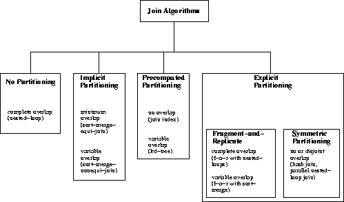
algorithms. Mishra and Eich identified four types of partitioning
employed by join algorithms [Mishra and Eich, 1992] :
- No Partitioning:
- The input relations
are not partitioned at all. They must be exhaustively compared in order
to find the tuple pairs that participate in the join.
- Implicit Partitioning:
-
Although the join algorithm does not have a specific step for
performing the partitioning, it does do some dividing or ordering
of the data in order to reduce the number of tuples to be compared
in the match stage.
- Explicit Partitioning:
-
The algorithm contains an explicit partitioning stage as part of
its execution.
- Precomputed Partitioning:
-
Partitioning is not performed as part of the actual join algorithm.
These techniques assume that some partitioning exists.
In addition to the type of partitioning, another important
characteristic is the mapping between the fragments of the input
relations. Let us assume the case of an equi-join  with
with
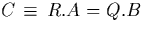 . Suppose that R and Q are divided into
their basic fragments
. Suppose that R and Q are divided into
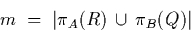
their basic fragments  and
and  respectively with m being the number of different values that
actually occur in the attributes R.A and Q.B. If we use the notation
of relational algebra
respectively with m being the number of different values that
actually occur in the attributes R.A and Q.B. If we use the notation
of relational algebra![[*]](foot_motif.gif) this means that
this means that
Imagine that the values in R.A and Q.B are  . A
basic fragment
. A
basic fragment  then holds
those tuples of R that hold xk as the value in attribute A,
i.e.
then holds
those tuples of R that hold xk as the value in attribute A,
i.e.
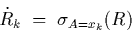
The  are defined accordingly. As an example for basic fragments
you might look at figure 3.13 where complete
partitioning created the basic fragments.
are defined accordingly. As an example for basic fragments
you might look at figure 3.13 where complete
partitioning created the basic fragments.
During the matching stage , each join algorithm
overlaps a basic fragment, say , with one or more basic
fragments of Q. The following degrees of overlap can be identified;
please note that the definitions differ slightly from those presented
in [Mishra and Eich, 1992] which is not clear enough in several aspects:
- Complete Overlap:
- In this case, a basic
fragment meets all basic fragments of Q. This happens in
the brute force nested-loops join (figure 3.6) or
the nested-loop join in conjunction with the
fragment-replicate-technique for parallelising a join
(figure 3.17).
- Minimum Overlap:
-
Tuples of meet all tuples of plus one tuple of
 and one of
  . This kind of overlap is
used in the sort-merge equi-join (figure 3.8).
. This kind of overlap is
used in the sort-merge equi-join (figure 3.8).
- No Overlap:
-
Tuples of only meet the tuples of , e.g. in
the completely partitioned hash join example of
figure 3.13.
- Disjoint Overlap:
-
This occurs when the definition of the `no-overlap-degree' is extended
to disjoint fragments, with a fragment being the union of basic
fragments. This means that tuples of a fragment, say
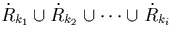 with
with 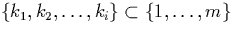 , meet tuples of the corresponding
fragment of Q, i.e.
, meet tuples of the corresponding
fragment of Q, i.e. 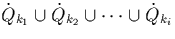 . This situation occurs in hash equi-joins
(figures 3.12, 3.13
and 3.20).
. This situation occurs in hash equi-joins
(figures 3.12, 3.13
and 3.20).
- Variable Overlap:
-
Tuples of meet tuples of and a varying number
of `neighbour fragments', i.e.
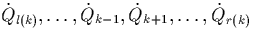 with
with 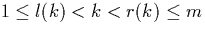 . We note that the values of l(k) and r(k) depend on k.
Variable overlaps occur in many index-based join algorithms, some
sort-merge nonequi-joins and sort-merge equi-joins in conjunction with
the fragment-and-replicate strategy (see
figure 3.18).
. We note that the values of l(k) and r(k) depend on k.
Variable overlaps occur in many index-based join algorithms, some
sort-merge nonequi-joins and sort-merge equi-joins in conjunction with
the fragment-and-replicate strategy (see
figure 3.18).
Table 3.1 summarises the relationships between
join techniques, types of partitioning and degrees of overlap. There
exists a certain duality between partitioning and overlap: no
partitioning, for example, imposes a complete overlap in the matching
stage. Explicit partitioning usually leads to a disjoint overlap and,
in the extreme case, to no overlap. Figure 3.21
shows the categorisation of join algorithms that arises from that.
We will use it in the following chapter when we discuss the implications
given by temporal join conditions.
Table:
Join algorithms, their type of partitioning and the degree
of overlap.
| Algorithm |
Type of Partitioning |
Degree of Overlap |
|---|
| nested-loop |
none |
complete |
| sort-merge equi-join |
implicit |
minimum |
| sort-merge nonequi-joins |
implicit |
minimum / variable |
| hash equi-join |
explicit |
disjoint / no |
| join index |
precomputed |
no |
| parallel equi-join |
explicit (symmetric) |
disjoint / no |
| parallel equi-join |
explicit (f-a-r) & no |
complete |
| parallel equi-join |
explicit (f-a-r) & implicit |
variable |
Figure:
Join algorithm categorisation.
 |
Next: Temporal Join Processing
Up: Join Processing
Previous: Symmetric Partitioning Technique
Thomas Zurek